Square Data Science Interview Questions

How to Build an Effective Remote Team

The Event-Driven Data Layer

Recently, I wrote an appeal to Adobe suggesting they implement first-party support for an event-driven data layer in Adobe Launch. I specifically mentioned an “event-driven, asynchronous data layer”. Let’s just call it the Event-Driven Data Layer (EDDL) to keep it simple. Since the article’s release, I’ve had a number of good conversations on this topic. The consensus seems to be that this is the right direction. For the purposes of keeping the article a manageable length, I didn’t go into too much detail of what an EDDL might look like. The goal of this article is to define what it is and why it’s a good thing.

Before we begin, let’s be clear about one thing. There’s an EDDL and a CEDDL.

CEDDL = Customer Experience Digital Data Layer. Legacy W3C.

EDDL = Event-Driven Data Layer. What this article is about.

I tried to find a less confusing abbreviation. Unfortunately, this one made the most sense. They’re both types of data layers. A good way to remember the difference is the CEDDL is 25% more cumbersome to spell and to implement. That’s being generous. The Event-Driven Data Layer describes what you’re implementing: a data layer that is constructed and transmitted to your TMS by events.

Let’s first walk through a concept that seems obvious but very few people care to think about. That is this: in a TMS, every tag is triggered by a some event. That means your pageview is triggered on an event. That event might be TMS Library Loaded (Page Top), DOM Ready, Window Loaded, or any other indication that the page has loaded. These are all events that happen on a page or screen. They are as much of an event as a click, mouseover, form submission, or anything else.

A pageview is a tag (think Adobe Analytics beacon). Viewing a page is an event. A custom link is a tag. Clicking a button is an event. Logging in is an event. Submitting a form is an event. That event might also be associated with some tags. Make sense? This is important because we need to abstract the tool from the data. Yes, you might choose to load Adobe Analytics pageview code when the window loads… but you COULD also choose to load a pageview on a click. The EDDL thinks independent of tool-specific definitions. Let’s dive into why this is the preferred method.

It’s harder to screw up

That doesn’t mean you can’t screw it up. It’s just harder to. You still need some code that sits in your header. The difference with the EDDL is:

1. It’s less code
2. You drop it in once and never have to touch it again

Maybe that means you’re simply declaring a variable (var foo = [];). Maybe it means you’re dropping in a little more code (copy/paste exercise). There’s no way around it – the variable or the function has to exist before you do anything with it. After that it’s all gravy. Timing is a non-issue with an EDDL. That’s because it proactively sends a message when a thing happens. Other data layer methodologies poll objects (like the Data Element Changed event). What does that mean?

Imagine you’re waiting on popular concert tickets to go on sale. You know what day they go on sale, but not what time. You know they’ll sell out fast, so you refresh Ticketmaster every half hour to see if their status changed. If you’re checking (or polling) to see if they’re for sale at 12:00 and they go on sale at 12:01, you might be out of luck. This is what’s called a race condition. After the status of the tickets change, you’re racing to see if you can get one before they’re gone.

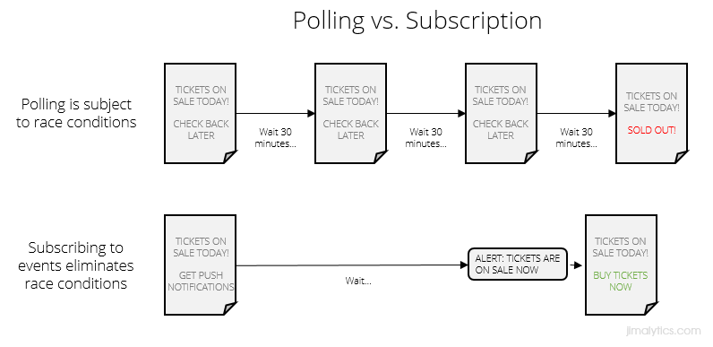
The same thing happens when you monitor data layers. If you go from Page A to Page B and you’re monitoring the object, there’s a very real chance you’ll be on the next page before your TMS realizes anything happened. That seriously sucks. You know what would fix this and save a lot of time? Subscribing to push notifications. Proactively tell me when the tickets are on sale. Don’t worry about loading the entire page object up-front. If we need to wait on servers, let me know when user information has propagated and then we’ll trigger a pageview. The EDDL uses these push notifications so you don’t have to worry about missing out on data.

It’s easier to communicate

Prioritization of data layers is difficult when it feels like a lot of work and its value isn’t immediately clear. Multiple code patterns paired with multiple sets of instructions feel like more work than one. We’re already taking focus away from the value of the data layer at this point.

The CEDDL requires teams to learn multiple concepts/patterns. There’s a page object… and then there are events. While it might be subconscious, multiple concepts/patterns (even simple ones) requires switching mental gears. They’re also both explained as though they’re different things. Here’s an example from Adobe where both the W3C and another methodology are recommended. If I’m not very technical or I’m new to analytics, this would make my head spin.

The EDDL is much simpler. You explain it once, use the same code pattern, and can be easily dropped into a template. Here’s how the documentation might look:

Data Layer Documentation

1.0: Page and User Information

Trigger: As soon as the information is available on each page loads or screen transition.

Code: dataLayer.push({“event”:“Page Loaded”,“page”:{…}…});

 

1.1: Email Submit

Trigger: When a user successfully submits an email address.

Code: dataLayer.push({“event”:“Email Submit”,“attributes”:{…}…});

The documentation is consistent. We aren’t suggesting page stuff is different from event stuff. Remember that pageviews are triggered via events, too. You won’t send a pageview until you have the data you need, either. You’re not trying to figure out whether you can cram it into the header, before Page Bottom, ahead of DOM Ready, or before Window Loaded. We can just say: “When the data is there, send the pageview.” A lot of companies opted out of the W3C CEDDL for this reason alone.

It’s just as comprehensive

You can literally create the W3C schema with it. An effective EDDL has some kind of computed state I can access that functions like any other JSON object. What does a computed state mean, exactly? In the context of data layers, it means the content that was passed into it is processed into some kind of comprehensive object. Let’s pretend we’re using dataLayer.push() and I’m pushing information into the data layer about the page and the user. This is a Single Page App, so we will want to dynamically replace the name of the page as the user navigates. Similar to Google Tag Manager, this pushes the page and user data into the dataLayer object (because dataLayer makes more sense than digitalData):

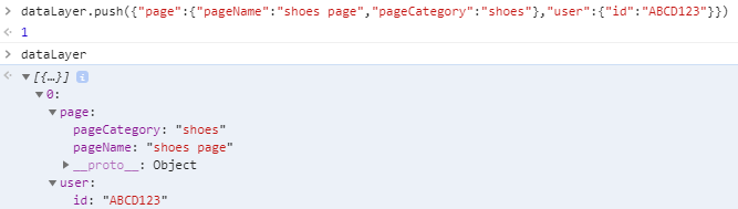
As a business user, it’s a bit of a stretch to learn how arrays work. I just want to see what the data looks like when the page loads so I know what I can work with. That’s where a computed state is useful. As a technical stakeholder, I can advise the business user to paste dataLayer.computedState into their console to see what data is available:

 

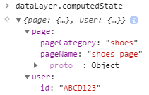
Looks like your average JSON object, right? Let’s see what happens when we want to change a field.

Side note: In hindsight, I probably should have named the pageCategory and pageName fields simply “category” and “name“. I’ll save naming convention recommendations for another post…

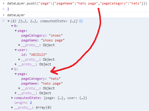
Here we’re just wanting to change the pageName and pageCategory fields. You can see the shoes data is still in that array above the hats page data. However, since that was the last information passed into the data layer, the computed state should update to reflect those changes:

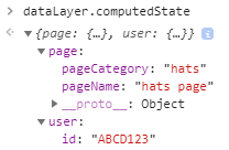
There you have it. I should have the ability to add data and clear out fields, as well. For those who aren’t as technical, please note that this computed state stuff is NOT functionality baked into dataLayer.push() by default. I did some extra work to manually create the computedState object. This is for modeling purposes only. Also note that a key differentiation between this and GTM’s data layer is a publicly exposed computed state. GTM does retain a computed state, but isn’t (easily) accessible via your console.

With this functionality, the EDDL is more capable and accessible than any other client-side data layer technique.

Final Thoughts

One reason people don’t implement data layers is because it’s intimidating. You’re part of a large organization with many stakeholders. Maintaining data layer standards takes work. You’re right. Let’s also acknowledge that maintaining anything is hard and requires a certain level of discipline. There’s turnover on your team. Developers cycle in and out. Oh, by the way – you have to get this stuff prioritized, too!

The Event-Driven Data Layer is easier to document. It’s easier to implement and not as vulnerable to timing issues. It’s what a minority of sophisticated companies have already built for themselves (100 different ways) and what the majority needs to adopt. This data layer supports any schema you want. If you like how the W3C is structured, build it. If not, don’t.

One critical piece you’ll notice I didn’t link you to some EDDL library. All of this information reflects how an EDDL should behave. There are many EDDLs out there and there won’t likely be one single standard. However, Event-Driven Data Layers will eventually replace the CEDDL model. It makes more sense. I will commit to settling on a single recommendation in the coming months. There are a few examples out there:

1. Google Tag Manager
2. Data Layer Manager

If you have a public-facing event-driven data layer framework, add a comment or message me on Twitter and I would be happy to add it to this list. In the meantime, if you’re working on a data layer – don’t let the lack of a “standard” stop you from building one. If you want to use the CEDDL, go for it! Having a data layer is better than not having one.

DataTau published first on DataTau

Architectural Innovations in Convolutional Neural Networks for Image Classification

A Gentle Introduction to the Innovations in LeNet, AlexNet, VGG, Inception, and ResNet Convolutional Neural Networks.

Convolutional neural networks are comprised of two very simple elements, namely convolutional layers and pooling layers.

Although simple, there are near-infinite ways to arrange these layers for a given computer vision problem.

Fortunately, there are both common patterns for configuring these layers and architectural innovations that you can use in order to develop very deep convolutional neural networks. Studying these architectural design decisions developed for state-of-the-art image classification tasks can provide both a rationale and intuition for how to use these designs when designing your own deep convolutional neural network models.

In this tutorial, you will discover the key architecture milestones for the use of convolutional neural networks for challenging image classification problems.

After completing this tutorial, you will know:

• How to pattern the number of filters and filter sizes when implementing convolutional neural networks.
• How to arrange convolutional and pooling layers in a uniform pattern to develop well-performing models.
• How to use the inception module and residual module to develop much deeper convolutional networks.

Let’s get started.

Tutorial Overview

This tutorial is divided into six parts; they are:

1. Architectural Design for CNNs
2. LeNet-5
3. AlexNet
4. VGG
5. Inception and GoogLeNet
6. Residual Network or ResNet

Architectural Design for CNNs

The elements of a convolutional neural network, such as convolutional and pooling layers, are relatively straightforward to understand.

The challenging part of using convolutional neural networks in practice is how to design model architectures that best use these simple elements.

A useful approach to learning how to design effective convolutional neural network architectures is to study successful applications. This is particularly straightforward to do because of the intense study and application of CNNs through 2012 to 2016 for the ImageNet Large Scale Visual Recognition Challenge, or ILSVRC. This challenge resulted in both the rapid advancement in the state of the art for very difficult computer vision tasks and the development of general innovations in the architecture of convolutional neural network models.

We will begin with the LeNet-5 that is often described as the first successful and important application of CNNs prior to the ILSVRC, then look at four different winning architectural innovations for the convolutional neural network developed for the ILSVRC, namely, AlexNet, VGG, Inception, and ResNet.

By understanding these milestone models and their architecture or architectural innovations from a high-level, you will develop both an appreciation for the use of these architectural elements in modern applications of CNN in computer vision, and be able to identify and choose architecture elements that may be useful in the design of your own models.

Want Results with Deep Learning for Computer Vision?

Take my free 7-day email crash course now (with sample code).

Click to sign-up and also get a free PDF Ebook version of the course.

Download Your FREE Mini-Course

LeNet-5

Perhaps the first widely known and successful application of convolutional neural networks was LeNet-5, described by Yann LeCun, et al. in their 1998 paper titled “Gradient-Based Learning Applied to Document Recognition” (get the PDF).

The system was developed for use in a handwritten character recognition problem and demonstrated on the MNIST standard dataset, achieving approximately 99.2% classification accuracy (or a 0.8% error rate). The network was then described as the central technique in a broader system referred to as Graph Transformer Networks.

It is a long paper, and perhaps the best part to focus on is Section II. B. that describes the LeNet-5 architecture. In the section, the paper describes the network as having seven layers with input grayscale images having the shape 32×32, the size of images in the MNIST dataset.

The model proposes a pattern of a convolutional layer followed by an average pooling layer, referred to as a subsampling layer. This pattern is repeated two and a half times before the output feature maps are flattened and fed to a number of fully connected layers for interpretation and a final prediction. A picture of the network architecture is provided in the paper and reproduced below.

Architecture of the LeNet-5 Convolutional Neural Network for Handwritten Character Recognition (taken from the 1998 paper).

The pattern of blocks of convolutional layers and pooling layers grouped together and repeated remains a common pattern in designing and using convolutional neural networks today, more than twenty years later.

Interestingly, the architecture uses a small number of filters with a very large size as the first hidden layer, specifically six filters each with the size of 28×28 pixels. After pooling, another convolutional layer has many more filters, again with a large size but smaller than the prior convolutional layer, specifically 16 filters with a size of 10×10 pixels, again followed by pooling. In the repetition of these two blocks of convolution and pooling layers, the trend is a decrease in the size of the filters, but an increase in the number of filters.

Compared to modern applications, the size of the filters is very large, as it is common to use 3×3 or similarly sized filter, and the number of filters is also small, but the trend of increasing the number of filters with the depth of the network also remains a common pattern in modern usage of the technique.

The third convolutional layer follows the first two blocks with 16 filters with a much smaller size of 5×5, although interestingly this is not followed by a pooling layer. The flattening of the feature maps and interpretation and classification of the extracted features by fully connected layers also remains a common pattern today. In modern terminology, the final section of the architecture is often referred to as the classifier, whereas the convolutional and pooling layers earlier in the model are referred to as the feature extractor.

We can summarize the key aspects of the architecture relevant in modern models as follows:

• Fixed-sized input images.
• Group convolutional and pooling layers into blocks.
• Repetition of convolutional-pooling blocks in the architecture.
• Increase in the number of features with the depth of the network.
• Distinct feature extraction and classifier parts of the architecture.

AlexNet

The work that perhaps could be credited with sparking renewed interest in neural networks and the beginning of the dominance of deep learning in many computer vision applications was the 2012 paper by Alex Krizhevsky, et al. titled “ImageNet Classification with Deep Convolutional Neural Networks.”

The paper describes a model later referred to as “AlexNet” designed to address the ImageNet Large Scale Visual Recognition Challenge or ILSVRC-2010 competition for classifying photographs of objects into one of 1,000 different categories.

The ILSVRC was a competition held from 2011 to 2016, designed to spur innovation in the field of computer vision. Before the development of AlexNet, the task was thought very difficult and far beyond the capability of modern computer vision methods. AlexNet successfully demonstrated the capability of the convolutional neural network model in the domain, and kindled a fire that resulted in many more improvements and innovations, many demonstrated on the same ILSVRC task in subsequent years. More broadly, the paper showed that it is possible to develop deep and effective end-to-end models for a challenging problem without using unsupervised pretraining techniques that were popular at the time.

Important in the design of AlexNet was a suite of methods that were new or successful, but not widely adopted at the time. Now, they have become requirements when using CNNs for image classification.

AlexNet made use of the rectified linear activation function, or ReLU, as the nonlinearly after each convolutional layer, instead of S-shaped functions such as the logistic or tanh that were common up until that point. Also, a softmax activation function was used in the output layer, now a staple for multi-class classification with neural networks.

The average pooling used in LeNet-5 was replaced with a max pooling method, although in this case, overlapping pooling was found to outperform non-overlapping pooling that is commonly used today (e.g. stride of pooling operation is the same size as the pooling operation, e.g. 2 by 2 pixels). To address overfitting, the newly proposed dropout method was used between the fully connected layers of the classifier part of the model to improve generalization error.

The architecture of AlexNet is deep and extends upon some of the patterns established with LeNet-5. The image below, taken from the paper, summarizes the model architecture, in this case, split into two pipelines to train on the GPU hardware of the time.

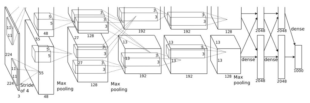
Architecture of the AlexNet Convolutional Neural Network for Object Photo Classification (taken from the 2012 paper).

The model has five convolutional layers in the feature extraction part of the model and three fully connected layers in the classifier part of the model.

Input images were fixed to the size 224×224 with three color channels. In terms of the number of filters used in each convolutional layer, the pattern of increasing the number of filters with depth seen in LeNet was mostly adhered to, in this case, the sizes: 96, 256, 384, 384, and 256. Similarly, the pattern of decreasing the size of the filter (kernel) with depth was used, starting from the smaller size of 11×11 and decreasing to 5×5, and then to 3×3 in the deeper layers. Use of small filters such as 5×5 and 3×3 is now the norm.

A pattern of a convolutional layer followed by pooling layer was used at the start and end of the feature detection part of the model. Interestingly, a pattern of convolutional layer followed immediately by a second convolutional layer was used. This pattern too has become a modern standard.

The model was trained with data augmentation, artificially increasing the size of the training dataset and giving the model more of an opportunity to learn the same features in different orientations.

We can summarize the key aspects of the architecture relevant in modern models as follows:

• Use of the ReLU activation function after convolutional layers and softmax for the output layer.
• Use of Max Pooling instead of Average Pooling.
• Use of Dropout regularization between the fully connected layers.
• Pattern of convolutional layer fed directly to another convolutional layer.
• Use of Data Augmentation.

VGG

The development of deep convolutional neural networks for computer vision tasks appeared to be a little bit of a dark art after AlexNet.

An important work that sought to standardize architecture design for deep convolutional networks and developed much deeper and better performing models in the process was the 2014 paper titled “Very Deep Convolutional Networks for Large-Scale Image Recognition” by Karen Simonyan and Andrew Zisserman.

Their architecture is generally referred to as VGG after the name of their lab, the Visual Geometry Group at Oxford. Their model was developed and demonstrated on the sameILSVRC competition, in this case, the ILSVRC-2014 version of the challenge.

The first important difference that has become a de facto standard is the use of a large number of small filters. Specifically, filters with the size 3×3 and 1×1 with the stride of one, different from the large sized filters in LeNet-5 and the smaller but still relatively large filters and large stride of four in AlexNet.

Max pooling layers are used after most, but not all, convolutional layers, learning from the example in AlexNet, yet all pooling is performed with the size 2×2 and the same stride, that too has become a de facto standard. Specifically, the VGG networks use examples of two, three, and even four convolutional layers stacked together before a max pooling layer is used. The rationale was that stacked convolutional layers with smaller filters approximate the effect of one convolutional layer with a larger sized filter, e.g. three stacked convolutional layers with 3×3 filters approximates one convolutional layer with a 7×7 filter.

Another important difference is the very large number of filters used. The number of filters increases with the depth of the model, although starts at a relatively large number of 64 and increases through 128, 256, and 512 filters at the end of the feature extraction part of the model.

A number of variants of the architecture were developed and evaluated, although two are referred to most commonly given their performance and depth. They are named for the number of layers: they are the VGG-16 and the VGG-19 for 16 and 19 learned layers respectively.

Below is a table taken from the paper; note the two far right columns indicating the configuration (number of filters) used in the VGG-16 and VGG-19 versions of the architecture.

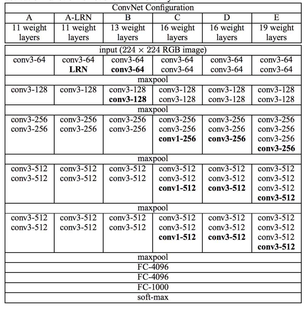
Architecture of the VGG Convolutional Neural Network for Object Photo Classification (taken from the 2014 paper).

The design decisions in the VGG models have become the starting point for simple and direct use of convolutional neural networks in general.

Finally, the VGG work was among the first to release the valuable model weights under a permissive license that led to a trend among deep learning computer vision researchers. This, in turn, has led to the heavy use of pre-trained models like VGG in transfer learning as a starting point on new computer vision tasks.

We can summarize the key aspects of the architecture relevant in modern models as follows:

• Use of very small convolutional filters, e.g. 3×3 and 1×1 with a stride of one.
• Use of max pooling with a size of 2×2 and a stride of the same dimensions.
• The importance of stacking convolutional layers together before using a pooling layer to define a block.
• Dramatic repetition of the convolutional-pooling block pattern.
• Development of very deep (16 and 19 layer) models.

Inception and GoogLeNet

Important innovations in the use of convolutional layers were proposed in the 2015 paper by Christian Szegedy, et al. titled “Going Deeper with Convolutions.”

In the paper, the authors propose an architecture referred to as inception (or inception v1 to differentiate it from extensions) and a specific model called GoogLeNet that achieved top results in the 2014 version of the ILSVRC challenge.

The key innovation on the inception models is called the inception module. This is a block of parallel convolutional layers with different sized filters (e.g. 1×1, 3×3, 5×5) and a 3×3 max pooling layer, the results of which are then concatenated. Below is an example of the inception module taken from the paper.

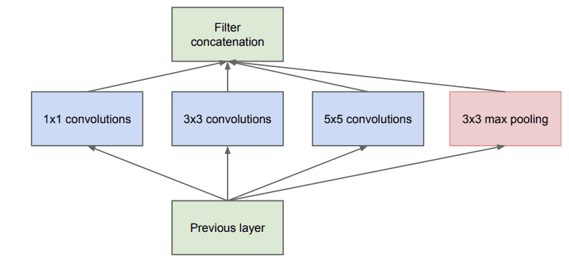
Example of the Naive Inception Module (taken from the 2015 paper).

A problem with a naive implementation of the inception model is that the number of filters (depth or channels) begins to build up fast, especially when inception modules are stacked.

Performing convolutions with larger filter sizes (e.g. 3 and 5) can be computationally expensive on a large number of filters. To address this, 1×1 convolutional layers are used to reduce the number of filters in the inception model. Specifically before the 3×3 and 5×5 convolutional layers and after the pooling layer. The image below taken from the paper shows this change to the inception module.

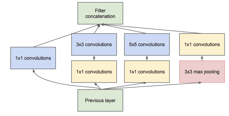
Example of the Inception Module With Dimensionality Reduction (taken from the 2015 paper).

A second important design decision in the inception model was connecting the output at different points in the model. This was achieved by creating small off-shoot output networks from the main network that were trained to make a prediction. The intent was to provide an additional error signal from the classification task at different points of the deep model in order to address the vanishing gradients problem. These small output networks were then removed after training.

Below shows a rotated version (left-to-right for input-to-output) of the architecture of the GoogLeNet model taken from the paper using the Inception modules from the input on the left to the output classification on the right and the two additional output networks that were only used during training.

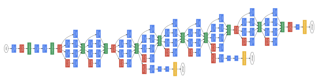
Architecture of the GoogLeNet Model Used During Training for Object Photo Classification (taken from the 2015 paper).

Interestingly, overlapping max pooling was used and a large average pooling operation was used at the end of the feature extraction part of the model prior to the classifier part of the model.

We can summarize the key aspects of the architecture relevant in modern models as follows:

• Development and repetition of the Inception module.
• Heavy use of the 1×1 convolution to reduce the number of channels.
• Use of error feedback at multiple points in the network.
• Development of very deep (22-layer) models.
• Use of global average pooling for the output of the model.

Residual Network or ResNet

A final important innovation in convolutional neural nets that we will review was proposed by Kaiming He, et al. in their 2016 paper titled “Deep Residual Learning for Image Recognition.”

In the paper, the authors proposed a very deep model called a Residual Network, or ResNet for short, an example of which achieved success on the 2015 version of the ILSVRC challenge.

Their model had an impressive 152 layers. Key to the model design is the idea of residual blocks that make use of shortcut connections. These are simply connections in the network architecture where the input is kept as-is (not weighted) and passed on to a deeper layer, e.g. skipping the next layer.

A residual block is a pattern of two convolutional layers with ReLU activation where the output of the block is combined with the input to the block, e.g. the shortcut connection. A projected version of the input used via 1×1 if the shape of the input to the block is different to the output of the block, so-called 1×1 convolutions. These are referred to as projected shortcut connections, compared to the unweighted or identity shortcut connections.

The authors start with what they call a plain network, which is a VGG-inspired deep convolutional neural network with small filters (3×3), grouped convolutional layers followed with no pooling in between, and an average pooling at the end of the feature detector part of the model prior to the fully connected output layer with a softmax activation function.

The plain network is modified to become a residual network by adding shortcut connections in order to define residual blocks. Typically the shape of the input for the shortcut connection is the same size as the output of the residual block.

The image below was taken from the paper and from left to right compares the architecture of a VGG model, a plain convolutional model, and a version of the plain convolutional with residual modules, called a residual network.

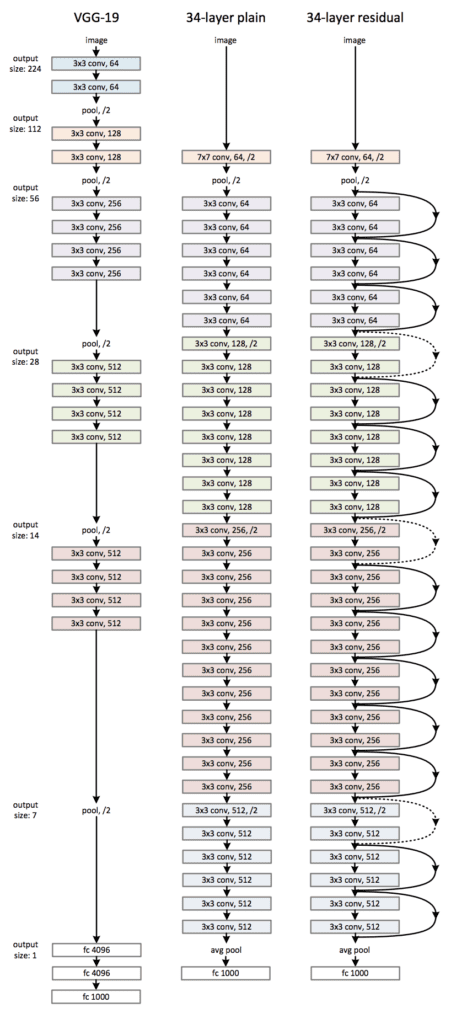
Architecture of the Residual Network for Object Photo Classification (taken from the 2016 paper).

We can summarize the key aspects of the architecture relevant in modern models as follows:

• Use of shortcut connections.
• Development and repetition of the residual blocks.
• Development of very deep (152-layer) models.

Further Reading

This section provides more resources on the topic if you are looking to go deeper.

Papers

• Gradient-based learning applied to document recognition, (PDF) 1998.
• ImageNet Classification with Deep Convolutional Neural Networks, 2012.
• Very Deep Convolutional Networks for Large-Scale Image Recognition, 2014.
• Going Deeper with Convolutions, 2015.
• Deep Residual Learning for Image Recognition, 2016

API

• Keras Applications API

Articles

• The 9 Deep Learning Papers You Need To Know About
• A Simple Guide to the Versions of the Inception Network, 2018.
• CNN Architectures: LeNet, AlexNet, VGG, GoogLeNet, ResNet and more., 2017.

Summary

In this tutorial, you discovered the key architecture milestones for the use of convolutional neural networks for challenging image classification.

Specifically, you learned:

• How to pattern the number of filters and filter sizes when implementing convolutional neural networks.
• How to arrange convolutional and pooling layers in a uniform pattern to develop well-performing models.
• How to use the inception module and residual module to develop much deeper convolutional networks.

Do you have any questions?
Ask your questions in the comments below and I will do my best to answer.

The post Architectural Innovations in Convolutional Neural Networks for Image Classification appeared first on Machine Learning Mastery.

Machine Learning Mastery published first on Machine Learning Mastery

Quiz Show Scandals/Admissions Scandal/Stormy Daniels/Beer names:being a lawyer would drive me nuts!!!!!!

0) Charles van Doren (see here) passed away recently. For those who don't know he he was (prob most of you) he was one of the contestants involved in RIGGED quiz shows in the 1950's.  While there was a Grand Jury Hearing about Quiz Shows being rigged, nobody went to jail since TV was new and it was not clear if rigging quiz shows was illegal. Laws were then passed to make them it illegal.

So why are today's so-called reality shows legal? I ask non-rhetorically.

(The person he beat in a rigged game show- Herb Stempel (see here) is still alive.)

1) The college admissions scandal. I won't restate the details and how awful it is since you can get that elsewhere and I doubt I can add much to it.  One thing I've heard in the discussions about it is a question that is often posted rhetorically but I want to pose for real:

There are people whose parents give X dollars to a school and they get admitted even though they are not qualified. Why is that legal?

I ask that question without an ax to grind and without anger. Why is out-right bribery of this sort legal?

Possibilities:

a) Its transparent. So being honest about bribery makes it okay?

b) My question said `even though they are not qualified' - what if they explicitly or implicitly said `having parents give money to our school is one of our qualifications'

c) The money they give is used to fund scholarships for students who can't afford to go. This is an argument for why its not immoral, not why its not illegal.

But here is my question: Really, what is the legal issue here? It still seems like bribery.

2) Big Oil gives money to congressman Smith, who then votes against a carbon tax. This seems like outright bribery

Caveat:

a) If Congressman Smith is normally a anti-regulation then he could say correctly that he was given the money because they agree with his general philosophy, so it's  not bribery.

b) If Congressman smith is normally pro-environment and has no problem with voting for taxes then perhaps it is bribery.

3) John Edwards a while back and Donald Trump now are claiming (not quite) that the money used to pay off their mistress to be quiet is NOT a campaign contribution, but was to keep the affair from his wife. (I don't think Donald Trump has admitted the affair so its harder to know what his defense is). But lets take a less controversial example of `what is a campaign contribution'

I throw a party for my wife's 50th birthday and I invite Beto O'Rourke and many voters and some Dem party big-wigs to the party. The party costs me $50,000.  While I claim it's for my wife's bday it really is for Beto to make connections to voters and others. So is that a campaign contribution?

4) The creators of HUGE ASS BEER are suing GIANT ASS BEER for trademark infringement. I am not making this up- see here

---------------------------------------------------------

All of these cases involve ill defined questions (e.g., `what is a bribe'). And the people arguing either side are not unbiased. The cases also illustrate why I prefer mathematics: nice clean questions that (for the most part) have answers. We may have our biases as to which way they go, but if it went the other way we would not sue in a court of law.
Computational Complexity published first on Computational Complexity

End of term

We’ve reached the end of term again on The Morning Paper, and I’ll be taking a two week break. The Morning Paper will resume on Tuesday 7th May (since Monday 6th is a public holiday in the UK).

My end of term tradition is to highlight a few of the papers from the term that I especially enjoyed, but this time around I want to let one work stand alone:

• Making reliable distributed systems in the presence of software errors, Joe Armstrong, December 2003.

You might also enjoy “The Mess We’re In,” and Joe’s seven deadly sins of programming:

1. Code even you cannot understand a week after you wrote it – no comments
2. Code with no specifications
3. Code that is shipped as soon as it runs and before it is beautiful
4. Code with added features
5. Code that is very very fast very very very obscure and incorrect
6. Code that is not beautiful
7. Code that you wrote without understanding the problem

We’re in an even bigger mess without you Joe. Thank you for everything. RIP.

the morning paper published first on the morning paper

A Gentle Introduction to Pooling Layers for Convolutional Neural Networks

Convolutional layers in a convolutional neural network summarize the presence of features in an input image.

A problem with the output feature maps is that they are sensitive to the location of the features in the input. One approach to address this sensitivity is to down sample the feature maps. This has the effect of making the resulting down sampled feature maps more robust to changes in the position of the feature in the image, referred to by the technical phrase “local translation invariance.”

Pooling layers provide an approach to down sampling feature maps by summarizing the presence of features in patches of the feature map. Two common pooling methods are average pooling and max pooling that summarize the average presence of a feature and the most activated presence of a feature respectively.

In this tutorial, you will discover how the pooling operation works and how to implement it in convolutional neural networks.

After completing this tutorial, you will know:

• Pooling is required to down sample the detection of features in feature maps.
• How to calculate and implement average and maximum pooling in a convolutional neural network.
• How to use global pooling in a convolutional neural network.

Let’s get started.

A Gentle Introduction to Pooling Layers for Convolutional Neural Networks
Photo by Nicholas A. Tonelli, some rights reserved.

Tutorial Overview

This tutorial is divided into five parts; they are:

1. Pooling
2. Detecting Vertical Lines
3. Average Pooling Layers
4. Max Pooling Layers
5. Global Pooling Layers

Want Results with Deep Learning for Computer Vision?

Take my free 7-day email crash course now (with sample code).

Click to sign-up and also get a free PDF Ebook version of the course.

Download Your FREE Mini-Course

Pooling Layers

Convolutional layers in a convolutional neural network systematically apply learned filters to input images in order to create feature maps that summarize the presence of those features in the input.

Convolutional layers prove very effective, and stacking convolutional layers in deep models allows layers close to the input to learn low-level features (e.g. lines) and layers deeper in the model to learn high-order or more abstract features, like shapes or specific objects.

A limitation of the feature map output of convolutional layers is that they record the precise position of features in the input. This means that small movements in the position of the feature in the input image will result in a different feature map. This can happen with re-cropping, rotation, shifting, and other minor changes to the input image.

A common approach to addressing this problem from signal processing is called down sampling. This is where a lower resolution version of an input signal is created that still contains the large or important structural elements, without the fine detail that may not be as useful to the task.

Down sampling can be achieved with convolutional layers by changing the stride of the convolution across the image. A more robust and common approach is to use a pooling layer.

A pooling layer is a new layer added after the convolutional layer. Specifically, after a nonlinearity (e.g. ReLU) has been applied to the feature maps output by a convolutional layer; for example the layers in a model may look as follows:

1. Input Image
2. Convolutional Layer
3. Nonlinearity
4. Pooling Layer

The addition of a pooling layer after the convolutional layer is a common pattern used for ordering layers within a convolutional neural network that may be repeated one or more times in a given model.

The pooling layer operates upon each feature map separately to create a new set of the same number of pooled feature maps.

Pooling involves selecting a pooling operation, much like a filter to be applied to feature maps. The size of the pooling operation or filter is smaller than the size of the feature map; specifically, it is almost always 2×2 pixels applied with a stride of 2 pixels.

This means that the pooling layer will always reduce the size of each feature map by a factor of 2, e.g. each dimension is halved, reducing the number of pixels or values in each feature map to one quarter the size. For example, a pooling layer applied to a feature map of 6×6 (36 pixels) will result in an output pooled feature map of 3×3 (9 pixels).

The pooling operation is specified, rather than learned. Two common functions used in the pooling operation are:

• Average Pooling: Calculate the average value for each patch on the feature map.
• Maximum Pooling (or Max Pooling): Calculate the maximum value for each patch of the feature map.

The result of using a pooling layer and creating down sampled or pooled feature maps is a summarized version of the features detected in the input. They are useful as small changes in the location of the feature in the input detected by the convolutional layer will result in a pooled feature map with the feature in the same location. This capability added by pooling is called the model’s invariance to local translation.

In all cases, pooling helps to make the representation become approximately invariant to small translations of the input. Invariance to translation means that if we translate the input by a small amount, the values of most of the pooled outputs do not change.

— Page 342, Deep Learning, 2016.

Now that we are familiar with the need and benefit of pooling layers, let’s look at some specific examples.

Detecting Vertical Lines

Before we look at some examples of pooling layers and their effects, let’s develop a small example of an input image and convolutional layer to which we can later add and evaluate pooling layers.

In this example, we define a single input image or sample that has one channel and is an 8 pixel by 8 pixel square with all 0 values and a two-pixel wide vertical line in the center.

# define input data
data = [[0, 0, 0, 1, 1, 0, 0, 0],
                [0, 0, 0, 1, 1, 0, 0, 0],
                [0, 0, 0, 1, 1, 0, 0, 0],
                [0, 0, 0, 1, 1, 0, 0, 0],
                [0, 0, 0, 1, 1, 0, 0, 0],
                [0, 0, 0, 1, 1, 0, 0, 0],
                [0, 0, 0, 1, 1, 0, 0, 0],
                [0, 0, 0, 1, 1, 0, 0, 0]]
data = asarray(data)
data = data.reshape(1, 8, 8, 1)

Next, we can define a model that expects input samples to have the shape (8, 8, 1) and has a single hidden convolutional layer with a single filter with the shape of 3 pixels by 3 pixels.

A rectified linear activation function, or ReLU for short, is then applied to each value in the feature map. This is a simple and effective nonlinearity, that in this case will not change the values in the feature map, but is present because we will later add subsequent pooling layers and pooling is added after the nonlinearity applied to the feature maps, e.g. a best practice.

# create model
model = Sequential()
model.add(Conv2D(1, (3,3), activation='relu', input_shape=(8, 8, 1)))
# summarize model
model.summary()

The filter is initialized with random weights as part of the initialization of the model.

Instead, we will hard code our own 3×3 filter that will detect vertical lines. That is the filter will strongly activate when it detects a vertical line and weakly activate when it does not. We expect that by applying this filter across the input image that the output feature map will show that the vertical line was detected.

# define a vertical line detector
detector = [[[[0]],[[1]],[[0]]],
            [[[0]],[[1]],[[0]]],
            [[[0]],[[1]],[[0]]]]
weights = [asarray(detector), asarray([0.0])]
# store the weights in the model
model.set_weights(weights)

Next, we can apply the filter to our input image by calling the predict() function on the model.

# apply filter to input data
yhat = model.predict(data)

The result is a four-dimensional output with one batch, a given number of rows and columns, and one filter, or [batch, rows, columns, filters]. We can print the activations in the single feature map to confirm that the line was detected.

# enumerate rows
for r in range(yhat.shape[1]):
        # print each column in the row
        print([yhat[0,r,c,0] for c in range(yhat.shape[2])])

Tying all of this together, the complete example is listed below.

# example of vertical line detection with a convolutional layer
from numpy import asarray
from keras.models import Sequential
from keras.layers import Conv2D
# define input data
data = [[0, 0, 0, 1, 1, 0, 0, 0],
                [0, 0, 0, 1, 1, 0, 0, 0],
                [0, 0, 0, 1, 1, 0, 0, 0],
                [0, 0, 0, 1, 1, 0, 0, 0],
                [0, 0, 0, 1, 1, 0, 0, 0],
                [0, 0, 0, 1, 1, 0, 0, 0],
                [0, 0, 0, 1, 1, 0, 0, 0],
                [0, 0, 0, 1, 1, 0, 0, 0]]
data = asarray(data)
data = data.reshape(1, 8, 8, 1)
# create model
model = Sequential()
model.add(Conv2D(1, (3,3), activation='relu', input_shape=(8, 8, 1)))
# summarize model
model.summary()
# define a vertical line detector
detector = [[[[0]],[[1]],[[0]]],
            [[[0]],[[1]],[[0]]],
            [[[0]],[[1]],[[0]]]]
weights = [asarray(detector), asarray([0.0])]
# store the weights in the model
model.set_weights(weights)
# apply filter to input data
yhat = model.predict(data)
# enumerate rows
for r in range(yhat.shape[1]):
        # print each column in the row
        print([yhat[0,r,c,0] for c in range(yhat.shape[2])])

Running the example first summarizes the structure of the model.

Of note is that the single hidden convolutional layer will take the 8×8 pixel input image and will produce a feature map with the dimensions of 6×6.

We can also see that the layer has 10 parameters: that is nine weights for the filter (3×3) and one weight for the bias.

Finally, the single feature map is printed.

We can see from reviewing the numbers in the 6×6 matrix that indeed the manually specified filter detected the vertical line in the middle of our input image.

_________________________________________________________________
Layer (type)                 Output Shape              Param #
=================================================================
conv2d_1 (Conv2D)            (None, 6, 6, 1)           10
=================================================================
Total params: 10
Trainable params: 10
Non-trainable params: 0
_________________________________________________________________

[0.0, 0.0, 3.0, 3.0, 0.0, 0.0]
[0.0, 0.0, 3.0, 3.0, 0.0, 0.0]
[0.0, 0.0, 3.0, 3.0, 0.0, 0.0]
[0.0, 0.0, 3.0, 3.0, 0.0, 0.0]
[0.0, 0.0, 3.0, 3.0, 0.0, 0.0]
[0.0, 0.0, 3.0, 3.0, 0.0, 0.0]

We can now look at some common approaches to pooling and how they impact the output feature maps.

Average Pooling Layer

On two-dimensional feature maps, pooling is typically applied in 2×2 patches of the feature map with a stride of (2,2).

Average pooling involves calculating the average for each patch of the feature map. This means that each 2×2 square of the feature map is down sampled to the average value in the square.

For example, the output of the line detector convolutional filter in the previous section was a 6×6 feature map. We can look at applying the average pooling operation to the first line of that feature map manually.

The first line for pooling (first two rows and six columns) of the output feature map were as follows:

[0.0, 0.0, 3.0, 3.0, 0.0, 0.0]
[0.0, 0.0, 3.0, 3.0, 0.0, 0.0]

The first pooling operation is applied as follows:

average(0.0, 0.0) = 0.0
        0.0, 0.0

Given the stride of two, the operation is moved along two columns to the left and the average is calculated:

average(3.0, 3.0) = 3.0
        3.0, 3.0

Again, the operation is moved along two columns to the left and the average is calculated:

average(0.0, 0.0) = 0.0
        0.0, 0.0

That’s it for the first line of pooling operations. The result is the first line of the average pooling operation:

[0.0, 3.0, 0.0]

Given the (2,2) stride, the operation would then be moved down two rows and back to the first column and the process continued.

Because the downsampling operation halves each dimension, we will expect the output of pooling applied to the 6×6 feature map to be a new 3×3 feature map. Given the horizontal symmetry of the feature map input, we would expect each row to have the same average pooling values. Therefore, we would expect the resulting average pooling of the detected line feature map from the previous section to look as follows:

[0.0, 3.0, 0.0]
[0.0, 3.0, 0.0]
[0.0, 3.0, 0.0]

We can confirm this by updating the example from the previous section to use average pooling.

This can be achieved in Keras by using the AveragePooling2D layer. The default pool_size (e.g. like the kernel size or filter size) of the layer is (2,2) and the default strides is None, which in this case means using the pool_size as the strides, which will be (2,2).

# create model
model = Sequential()
model.add(Conv2D(1, (3,3), activation='relu', input_shape=(8, 8, 1)))
model.add(AveragePooling2D())

The complete example with average pooling is listed below.

# example of average pooling
from numpy import asarray
from keras.models import Sequential
from keras.layers import Conv2D
from keras.layers import AveragePooling2D
# define input data
data = [[0, 0, 0, 1, 1, 0, 0, 0],
                [0, 0, 0, 1, 1, 0, 0, 0],
                [0, 0, 0, 1, 1, 0, 0, 0],
                [0, 0, 0, 1, 1, 0, 0, 0],
                [0, 0, 0, 1, 1, 0, 0, 0],
                [0, 0, 0, 1, 1, 0, 0, 0],
                [0, 0, 0, 1, 1, 0, 0, 0],
                [0, 0, 0, 1, 1, 0, 0, 0]]
data = asarray(data)
data = data.reshape(1, 8, 8, 1)
# create model
model = Sequential()
model.add(Conv2D(1, (3,3), activation='relu', input_shape=(8, 8, 1)))
model.add(AveragePooling2D())
# summarize model
model.summary()
# define a vertical line detector
detector = [[[[0]],[[1]],[[0]]],
            [[[0]],[[1]],[[0]]],
            [[[0]],[[1]],[[0]]]]
weights = [asarray(detector), asarray([0.0])]
# store the weights in the model
model.set_weights(weights)
# apply filter to input data
yhat = model.predict(data)
# enumerate rows
for r in range(yhat.shape[1]):
        # print each column in the row
        print([yhat[0,r,c,0] for c in range(yhat.shape[2])])

Running the example first summarizes the model.

We can see from the model summary that the input to the pooling layer will be a single feature map with the shape (6,6) and that the output of the average pooling layer will be a single feature map with each dimension halved, with the shape (3,3).

Applying the average pooling results in a new feature map that still detects the line, although in a down sampled manner, exactly as we expected from calculating the operation manually.

_________________________________________________________________
Layer (type)                 Output Shape              Param #
=================================================================
conv2d_1 (Conv2D)            (None, 6, 6, 1)           10
_________________________________________________________________
average_pooling2d_1 (Average (None, 3, 3, 1)           0
=================================================================
Total params: 10
Trainable params: 10
Non-trainable params: 0
_________________________________________________________________

[0.0, 3.0, 0.0]
[0.0, 3.0, 0.0]
[0.0, 3.0, 0.0]

Average pooling works well, although it is more common to use max pooling.

Max Pooling Layer

Maximum pooling, or max pooling, is a pooling operation that calculates the maximum, or largest, value in each patch of each feature map.

The results are down sampled or pooled feature maps that highlight the most present feature in the patch, not the average presence of the feature in the case of average pooling. This has been found to work better in practice than average pooling for computer vision tasks like image classification.

In a nutshell, the reason is that features tend to encode the spatial presence of some pattern or concept over the different tiles of the feature map (hence, the term feature map), and it’s more informative to look at the maximal presence of different features than at their average presence.

— Page 129, Deep Learning with Python, 2017.

We can make the max pooling operation concrete by again applying it to the output feature map of the line detector convolutional operation and manually calculate the first row of the pooled feature map.

The first line for pooling (first two rows and six columns) of the output feature map were as follows:

[0.0, 0.0, 3.0, 3.0, 0.0, 0.0]
[0.0, 0.0, 3.0, 3.0, 0.0, 0.0]

The first max pooling operation is applied as follows:

max(0.0, 0.0) = 0.0
    0.0, 0.0

Given the stride of two, the operation is moved along two columns to the left and the max is calculated:

max(3.0, 3.0) = 3.0
    3.0, 3.0

Again, the operation is moved along two columns to the left and the max is calculated:

max(0.0, 0.0) = 0.0
    0.0, 0.0

That’s it for the first line of pooling operations.

The result is the first line of the max pooling operation:

[0.0, 3.0, 0.0]

Again, given the horizontal symmetry of the feature map provided for pooling, we would expect the pooled feature map to look as follows:

[0.0, 3.0, 0.0]
[0.0, 3.0, 0.0]
[0.0, 3.0, 0.0]

It just so happens that the chosen line detector image and feature map produce the same output when downsampled with average pooling and maximum pooling.

The maximum pooling operation can be added to the worked example by adding the MaxPooling2D layer provided by the Keras API.

# create model
model = Sequential()
model.add(Conv2D(1, (3,3), activation='relu', input_shape=(8, 8, 1)))
model.add(MaxPooling2D())

The complete example of vertical line detection with max pooling is listed below.

# example of max pooling
from numpy import asarray
from keras.models import Sequential
from keras.layers import Conv2D
from keras.layers import MaxPooling2D
# define input data
data = [[0, 0, 0, 1, 1, 0, 0, 0],
                [0, 0, 0, 1, 1, 0, 0, 0],
                [0, 0, 0, 1, 1, 0, 0, 0],
                [0, 0, 0, 1, 1, 0, 0, 0],
                [0, 0, 0, 1, 1, 0, 0, 0],
                [0, 0, 0, 1, 1, 0, 0, 0],
                [0, 0, 0, 1, 1, 0, 0, 0],
                [0, 0, 0, 1, 1, 0, 0, 0]]
data = asarray(data)
data = data.reshape(1, 8, 8, 1)
# create model
model = Sequential()
model.add(Conv2D(1, (3,3), activation='relu', input_shape=(8, 8, 1)))
model.add(MaxPooling2D())
# summarize model
model.summary()
# define a vertical line detector
detector = [[[[0]],[[1]],[[0]]],
            [[[0]],[[1]],[[0]]],
            [[[0]],[[1]],[[0]]]]
weights = [asarray(detector), asarray([0.0])]
# store the weights in the model
model.set_weights(weights)
# apply filter to input data
yhat = model.predict(data)
# enumerate rows
for r in range(yhat.shape[1]):
        # print each column in the row
        print([yhat[0,r,c,0] for c in range(yhat.shape[2])])

Running the example first summarizes the model.

We can see, as we might expect by now, that the output of the max pooling layer will be a single feature map with each dimension halved, with the shape (3,3).

Applying the max pooling results in a new feature map that still detects the line, although in a down sampled manner.

_________________________________________________________________
Layer (type)                 Output Shape              Param #
=================================================================
conv2d_1 (Conv2D)            (None, 6, 6, 1)           10
_________________________________________________________________
max_pooling2d_1 (MaxPooling2 (None, 3, 3, 1)           0
=================================================================
Total params: 10
Trainable params: 10
Non-trainable params: 0
_________________________________________________________________

[0.0, 3.0, 0.0]
[0.0, 3.0, 0.0]
[0.0, 3.0, 0.0]

Global Pooling Layers

There is another type of pooling that is sometimes used called global pooling.

Instead of down sampling patches of the input feature map, global pooling down samples the entire feature map to a single value. This would be the same as setting the pool_size to the size of the input feature map.

Global pooling can be used in a model to aggressively summarize the presence of a feature in an image. It is also sometimes used in models as an alternative to using a fully connected layer to transition from feature maps to an output prediction for the model.

Both global average pooling and global max pooling are supported by Keras via the GlobalAveragePooling2D and GlobalMaxPooling2D classes respectively.

For example, we can add global max pooling to the convolutional model used for vertical line detection.

# create model
model = Sequential()
model.add(Conv2D(1, (3,3), activation='relu', input_shape=(8, 8, 1)))
model.add(GlobalMaxPooling2D())

The outcome will be a single value that will summarize the strongest activation or presence of the vertical line in the input image.

The complete code listing is provided below.

# example of using global max pooling
from numpy import asarray
from keras.models import Sequential
from keras.layers import Conv2D
from keras.layers import GlobalMaxPooling2D
# define input data
data = [[0, 0, 0, 1, 1, 0, 0, 0],
                [0, 0, 0, 1, 1, 0, 0, 0],
                [0, 0, 0, 1, 1, 0, 0, 0],
                [0, 0, 0, 1, 1, 0, 0, 0],
                [0, 0, 0, 1, 1, 0, 0, 0],
                [0, 0, 0, 1, 1, 0, 0, 0],
                [0, 0, 0, 1, 1, 0, 0, 0],
                [0, 0, 0, 1, 1, 0, 0, 0]]
data = asarray(data)
data = data.reshape(1, 8, 8, 1)
# create model
model = Sequential()
model.add(Conv2D(1, (3,3), activation='relu', input_shape=(8, 8, 1)))
model.add(GlobalMaxPooling2D())
# summarize model
model.summary()
# # define a vertical line detector
detector = [[[[0]],[[1]],[[0]]],
            [[[0]],[[1]],[[0]]],
            [[[0]],[[1]],[[0]]]]
weights = [asarray(detector), asarray([0.0])]
# store the weights in the model
model.set_weights(weights)
# apply filter to input data
yhat = model.predict(data)
# enumerate rows
print(yhat)

Running the example first summarizes the model

We can see that, as expected, the output of the global pooling layer is a single value that summarizes the presence of the feature in the single feature map.

Next, the output of the model is printed showing the effect of global max pooling on the feature map, printing the single largest activation.

_________________________________________________________________
Layer (type)                 Output Shape              Param #
=================================================================
conv2d_1 (Conv2D)            (None, 6, 6, 1)           10
_________________________________________________________________
global_max_pooling2d_1 (Glob (None, 1)                 0
=================================================================
Total params: 10
Trainable params: 10
Non-trainable params: 0
_________________________________________________________________

[[3.]]

Further Reading

This section provides more resources on the topic if you are looking to go deeper.

Posts

• Crash Course in Convolutional Neural Networks for Machine Learning

Books

• Chapter 9: Convolutional Networks, Deep Learning, 2016.
• Chapter 5: Deep Learning for Computer Vision, Deep Learning with Python, 2017.

API

• Keras Convolutional Layers API
• Keras Pooling Layers API

Summary

In this tutorial, you discovered how the pooling operation works and how to implement it in convolutional neural networks.

Specifically, you learned:

• Pooling is required to down sample the detection of features in feature maps.
• How to calculate and implement average and maximum pooling in a convolutional neural network.
• How to use global pooling in a convolutional neural network.

Do you have any questions?
Ask your questions in the comments below and I will do my best to answer.

The post A Gentle Introduction to Pooling Layers for Convolutional Neural Networks appeared first on Machine Learning Mastery.

Machine Learning Mastery published first on Machine Learning Mastery

Creating fun shapes in D3.js

Advanced NLP with SpaCy

Train models and run notebooks on AWS cheaper and simpler than with SageMaker

A Gentle Introduction to Padding and Stride for Convolutional Neural Networks

The convolutional layer in convolutional neural networks systematically applies filters to an input and creates output feature maps.

Although the convolutional layer is very simple, it is capable of achieving sophisticated and impressive results. Nevertheless, it can be challenging to develop an intuition for how the shape of the filters impacts the shape of the output feature map and how related configuration hyperparameters such as padding and stride should be configured.

In this tutorial, you will discover an intuition for filter size, the need for padding, and stride in convolutional neural networks.

After completing this tutorial, you will know:

• How filter size or kernel size impacts the shape of the output feature map.
• How the filter size creates a border effect in the feature map and how it can be overcome with padding.
• How the stride of the filter on the input image can be used to downsample the size of the output feature map.

Let’s get started.

A Gentle Introduction to Padding and Stride for Convolutional Neural Networks
Photo by Red~Star, some rights reserved.

Tutorial Overview

This tutorial is divided into five parts; they are:

1. Convolutional Layer
2. Problem of Border Effects
3. Effect of Filter Size (Kernel Size)
4. Fix the Border Effect Problem With Padding
5. Downsample Input With Stride

Want Results with Deep Learning for Computer Vision?

Take my free 7-day email crash course now (with sample code).

Click to sign-up and also get a free PDF Ebook version of the course.

Download Your FREE Mini-Course

Convolutional Layer

In a convolutional neural network, a convolutional layer is responsible for the systematic application of one or more filters to an input.

The multiplication of the filter to the input image results in a single output. The input is typically three-dimensional images (e.g. rows, columns and channels), and in turn, the filters are also three-dimensional with the same number of channels and fewer rows and columns than the input image. As such, the filter is repeatedly applied to each part of the input image, resulting in a two-dimensional output map of activations, called a feature map.

Keras provides an implementation of the convolutional layer called a Conv2D.

It requires that you specify the expected shape of the input images in terms of rows (height), columns (width), and channels (depth) or [rows, columns, channels].

The filter contains the weights that must be learned during the training of the layer. The filter weights represent the structure or feature that the filter will detect and the strength of the activation indicates the degree to which the feature was detected.

The layer requires that both the number of filters be specified and that the shape of the filters be specified.

We can demonstrate this with a small example. In this example, we define a single input image or sample that has one channel and is an eight pixel by eight pixel square with all 0 values and a two-pixel wide vertical line in the center.

# define input data
data = [[0, 0, 0, 1, 1, 0, 0, 0],
                [0, 0, 0, 1, 1, 0, 0, 0],
                [0, 0, 0, 1, 1, 0, 0, 0],
                [0, 0, 0, 1, 1, 0, 0, 0],
                [0, 0, 0, 1, 1, 0, 0, 0],
                [0, 0, 0, 1, 1, 0, 0, 0],
                [0, 0, 0, 1, 1, 0, 0, 0],
                [0, 0, 0, 1, 1, 0, 0, 0]]
data = asarray(data)
data = data.reshape(1, 8, 8, 1)

Next, we can define a model that expects input samples to have the shape (8, 8, 1) and has a single hidden convolutional layer with a single filter with the shape of three pixels by three pixels.

# create model
model = Sequential()
model.add(Conv2D(1, (3,3), input_shape=(8, 8, 1)))
# summarize model
model.summary()

The filter is initialized with random weights as part of the initialization of the model. We will overwrite the random weights and hard code our own 3×3 filter that will detect vertical lines.

That is the filter will strongly activate when it detects a vertical line and weakly activate when it does not. We expect that by applying this filter across the input image, the output feature map will show that the vertical line was detected.

# define a vertical line detector
detector = [[[[0]],[[1]],[[0]]],
            [[[0]],[[1]],[[0]]],
            [[[0]],[[1]],[[0]]]]
weights = [asarray(detector), asarray([0.0])]
# store the weights in the model
model.set_weights(weights)

Next, we can apply the filter to our input image by calling the predict() function on the model.

# apply filter to input data
yhat = model.predict(data)

The result is a four-dimensional output with one batch, a given number of rows and columns, and one filter, or [batch, rows, columns, filters].

We can print the activations in the single feature map to confirm that the line was detected.

# enumerate rows
for r in range(yhat.shape[1]):
        # print each column in the row
        print([yhat[0,r,c,0] for c in range(yhat.shape[2])])

Tying all of this together, the complete example is listed below.

# example of using a single convolutional layer
from numpy import asarray
from keras.models import Sequential
from keras.layers import Conv2D
# define input data
data = [[0, 0, 0, 1, 1, 0, 0, 0],
                [0, 0, 0, 1, 1, 0, 0, 0],
                [0, 0, 0, 1, 1, 0, 0, 0],
                [0, 0, 0, 1, 1, 0, 0, 0],
                [0, 0, 0, 1, 1, 0, 0, 0],
                [0, 0, 0, 1, 1, 0, 0, 0],
                [0, 0, 0, 1, 1, 0, 0, 0],
                [0, 0, 0, 1, 1, 0, 0, 0]]
data = asarray(data)
data = data.reshape(1, 8, 8, 1)
# create model
model = Sequential()
model.add(Conv2D(1, (3,3), input_shape=(8, 8, 1)))
# summarize model
model.summary()
# define a vertical line detector
detector = [[[[0]],[[1]],[[0]]],
            [[[0]],[[1]],[[0]]],
            [[[0]],[[1]],[[0]]]]
weights = [asarray(detector), asarray([0.0])]
# store the weights in the model
model.set_weights(weights)
# apply filter to input data
yhat = model.predict(data)
# enumerate rows
for r in range(yhat.shape[1]):
        # print each column in the row
        print([yhat[0,r,c,0] for c in range(yhat.shape[2])])

Running the example first summarizes the structure of the model.

Of note is that the single hidden convolutional layer will take the 8×8 pixel input image and will produce a feature map with the dimensions of 6×6. We will go into why this is the case in the next section.

We can also see that the layer has 10 parameters, that is nine weights for the filter (3×3) and one weight for the bias.

Finally, the feature map is printed. We can see from reviewing the numbers in the 6×6 matrix that indeed the manually specified filter detected the vertical line in the middle of our input image.

_________________________________________________________________
Layer (type)                 Output Shape              Param #
=================================================================
conv2d_1 (Conv2D)            (None, 6, 6, 1)           10
=================================================================
Total params: 10
Trainable params: 10
Non-trainable params: 0
_________________________________________________________________


[0.0, 0.0, 3.0, 3.0, 0.0, 0.0]
[0.0, 0.0, 3.0, 3.0, 0.0, 0.0]
[0.0, 0.0, 3.0, 3.0, 0.0, 0.0]
[0.0, 0.0, 3.0, 3.0, 0.0, 0.0]
[0.0, 0.0, 3.0, 3.0, 0.0, 0.0]
[0.0, 0.0, 3.0, 3.0, 0.0, 0.0]

Problem of Border Effects

In the previous section, we defined a single filter with the size of three pixels high and three pixels wide (rows, columns).

We saw that the application of the 3×3 filter, referred to as the kernel size in Keras, to the 8×8 input image resulted in a feature map with the size of 6×6.

That is, the input image with 64 pixels was reduced to a feature map with 36 pixels. Where did the other 28 pixels go?

The filter is applied systematically to the input image. It starts at the top left corner of the image and is moved from left to right one pixel column at a time until the edge of the filter reaches the edge of the image.

For a 3×3 pixel filter applied to a 8×8 input image, we can see that it can only be applied six times, resulting in the width of six in the output feature map.

For example, let’s work through each of the six patches of the input image (left) dot product (“.” operator) the filter (right):

0, 0, 0   0, 1, 0
0, 0, 0 . 0, 1, 0 = 0
0, 0, 0   0, 1, 0

Moved right one pixel:

0, 0, 1   0, 1, 0
0, 0, 1 . 0, 1, 0 = 0
0, 0, 1   0, 1, 0

Moved right one pixel:

0, 1, 1   0, 1, 0
0, 1, 1 . 0, 1, 0 = 3
0, 1, 1   0, 1, 0

Moved right one pixel:

1, 1, 0   0, 1, 0
1, 1, 0 . 0, 1, 0 = 3
1, 1, 0   0, 1, 0

Moved right one pixel:

1, 0, 0   0, 1, 0
1, 0, 0 . 0, 1, 0 = 0
1, 0, 0   0, 1, 0

Moved right one pixel:

0, 0, 0   0, 1, 0
0, 0, 0 . 0, 1, 0 = 0
0, 0, 0   0, 1, 0

That gives us the first row and each column of the output feature map:

0.0, 0.0, 3.0, 3.0, 0.0, 0.0

The reduction in the size of the input to the feature map is referred to as border effects. It is caused by the interaction of the filter with the border of the image.

This is often not a problem for large images and small filters but can be a problem with small images. It can also become a problem once a number of convolutional layers are stacked.

For example, below is the same model updated to have two stacked convolutional layers.

This means that a 3×3 filter is applied to the 8×8 input image to result in a 6×6 feature map as in the previous section. A 3×3 filter is then applied to the 6×6 feature map.

# example of stacked convolutional layers
from keras.models import Sequential
from keras.layers import Conv2D
# create model
model = Sequential()
model.add(Conv2D(1, (3,3), input_shape=(8, 8, 1)))
model.add(Conv2D(1, (3,3)))
# summarize model
model.summary()

Running the example summarizes the shape of the output from each layer.

We can see that the application of filters to the feature map output of the first layer, in turn, results in a smaller 4×4 feature map.

This can become a problem as we develop very deep convolutional neural network models with tens or hundreds of layers. We will simply run out of data in our feature maps upon which to operate.

_________________________________________________________________
Layer (type)                 Output Shape              Param #
=================================================================
conv2d_1 (Conv2D)            (None, 6, 6, 1)           10
_________________________________________________________________
conv2d_2 (Conv2D)            (None, 4, 4, 1)           10
=================================================================
Total params: 20
Trainable params: 20
Non-trainable params: 0
_________________________________________________________________

Effect of Filter Size (Kernel Size)

Different sized filters will detect different sized features in the input image and, in turn, will result in differently sized feature maps.

It is common to use 3×3 sized filters, and perhaps 5×5 or even 7×7 sized filters, for larger input images.

For example, below is an example of the model with a single filter updated to use a filter size of 5×5 pixels.

# example of a convolutional layer
from keras.models import Sequential
from keras.layers import Conv2D
# create model
model = Sequential()
model.add(Conv2D(1, (5,5), input_shape=(8, 8, 1)))
# summarize model
model.summary()

Running the example demonstrates that the 5×5 filter can only be applied to the 8×8 input image 4 times, resulting in a 4×4 feature map output.

_________________________________________________________________
Layer (type)                 Output Shape              Param #
=================================================================
conv2d_1 (Conv2D)            (None, 4, 4, 1)           26
=================================================================
Total params: 26
Trainable params: 26
Non-trainable params: 0
_________________________________________________________________

It may help to further develop the intuition of the relationship between filter size and the output feature map to look at two extreme cases.

The first is a filter with the size of 1×1 pixels.

# example of a convolutional layer
from keras.models import Sequential
from keras.layers import Conv2D
# create model
model = Sequential()
model.add(Conv2D(1, (1,1), input_shape=(8, 8, 1)))
# summarize model
model.summary()

Running the example demonstrates that the output feature map has the same size as the input, specifically 8×8. This is because the filter only has a single weight (and a bias).

_________________________________________________________________
Layer (type)                 Output Shape              Param #
=================================================================
conv2d_1 (Conv2D)            (None, 8, 8, 1)           2
=================================================================
Total params: 2
Trainable params: 2
Non-trainable params: 0
_________________________________________________________________

The other extreme is a filter with the same size as the input, in this case, 8×8 pixels.

# example of a convolutional layer
from keras.models import Sequential
from keras.layers import Conv2D
# create model
model = Sequential()
model.add(Conv2D(1, (8,8), input_shape=(8, 8, 1)))
# summarize model
model.summary()

Running the example, we can see that, as you might expect, there is one weight for each pixel in the input image (64 + 1 for the bias) and that the output is a feature map with a single pixel.

_________________________________________________________________
Layer (type)                 Output Shape              Param #
=================================================================
conv2d_1 (Conv2D)            (None, 1, 1, 1)           65
=================================================================
Total params: 65
Trainable params: 65
Non-trainable params: 0
_________________________________________________________________

Now that we are familiar with the effect of filter sizes on the size of the resulting feature map, let’s look at how we can stop losing pixels.

Fix the Border Effect Problem With Padding

By default, a filter starts at the left of the image with the left-hand side of the filter sitting on the far left pixels of the image. The filter is then stepped across the image one column at a time until the right-hand side of the filter is sitting on the far right pixels of the image.

An alternative approach to applying a filter to an image is to ensure that each pixel in the image is given an opportunity to be at the center of the filter.

By default, this is not the case, as the pixels on the edge of the input are only ever exposed to the edge of the filter. By starting the filter outside the frame of the image, it gives the pixels on the border of the image more of an opportunity for interacting with the filter, more of an opportunity for features to be detected by the filter, and in turn, an output feature map that has the same shape as the input image.

For example, in the case of applying a 3×3 filter to the 8×8 input image, we can add a border of one pixel around the outside of the image. This has the effect of artificially creating a 10×10 input image. When the 3×3 filter is applied, it results in an 8×8 feature map. The added pixel values could have the value zero value that has no effect with the dot product operation when the filter is applied.

x, x, x   0, 1, 0
x, 0, 0 . 0, 1, 0 = 0
x, 0, 0   0, 1, 0

The addition of pixels to the edge of the image is called padding.

In Keras, this is specified via the “padding” argument on the Conv2D layer, which has the default value of ‘valid‘ (no padding). This means that the filter is applied only to valid ways to the input.

The ‘padding‘ value of ‘same‘ calculates and adds the padding required to the input image (or feature map) to ensure that the output has the same shape as the input.

The example below adds padding to the convolutional layer in our worked example.

# example a convolutional layer with padding
from keras.models import Sequential
from keras.layers import Conv2D
# create model
model = Sequential()
model.add(Conv2D(1, (3,3), padding='same', input_shape=(8, 8, 1)))
# summarize model
model.summary()

Running the example demonstrates that the shape of the output feature map is the same as the input image: that the padding had the desired effect.

_________________________________________________________________
Layer (type)                 Output Shape              Param #
=================================================================
conv2d_1 (Conv2D)            (None, 8, 8, 1)           10
=================================================================
Total params: 10
Trainable params: 10
Non-trainable params: 0
_________________________________________________________________

The addition of padding allows the development of very deep models in such a way that the feature maps do not dwindle away to nothing.

The example below demonstrates this with three stacked convolutional layers.

# example a deep cnn with padding
from keras.models import Sequential
from keras.layers import Conv2D
# create model
model = Sequential()
model.add(Conv2D(1, (3,3), padding='same', input_shape=(8, 8, 1)))
model.add(Conv2D(1, (3,3), padding='same'))
model.add(Conv2D(1, (3,3), padding='same'))
# summarize model
model.summary()

Running the example, we can see that with the addition of padding, the shape of the output feature maps remains fixed at 8×8 even three layers deep.

_________________________________________________________________
Layer (type)                 Output Shape              Param #
=================================================================
conv2d_1 (Conv2D)            (None, 8, 8, 1)           10
_________________________________________________________________
conv2d_2 (Conv2D)            (None, 8, 8, 1)           10
_________________________________________________________________
conv2d_3 (Conv2D)            (None, 8, 8, 1)           10
=================================================================
Total params: 30
Trainable params: 30
Non-trainable params: 0
_________________________________________________________________

Downsample Input With Stride

The filter is moved across the image left to right, top to bottom, with a one-pixel column change on the horizontal movements, then a one-pixel row change on the vertical movements.

The amount of movement between applications of the filter to the input image is referred to as the stride, and it is almost always symmetrical in height and width dimensions.

The default stride or strides in two dimensions is (1,1) for the height and the width movement, performed when needed. And this default works well in most cases.

The stride can be changed, which has an effect both on how the filter is applied to the image and, in turn, the size of the resulting feature map.

For example, the stride can be changed to (2,2). This has the effect of moving the filter two pixels left for each horizontal movement of the filter and two pixels down for each vertical movement of the filter when creating the feature map.

We can demonstrate this with an example using the 8×8 image with a vertical line (left) dot product (“.” operator) with the vertical line filter (right) with a stride of two pixels:

0, 0, 0   0, 1, 0
0, 0, 0 . 0, 1, 0 = 0
0, 0, 0   0, 1, 0

Moved right two pixels:

0, 1, 1   0, 1, 0
0, 1, 1 . 0, 1, 0 = 3
0, 1, 1   0, 1, 0

Moved right two pixels:

1, 0, 0   0, 1, 0
1, 0, 0 . 0, 1, 0 = 0
1, 0, 0   0, 1, 0

We can see that there are only three valid applications of the 3×3 filters to the 8×8 input image with a stride of two. This will be the same in the vertical dimension.

This has the effect of applying the filter in such a way that the normal feature map output (6×6) is down-sampled so that the size of each dimension is reduced by half (3×3), resulting in 1/4 the number of pixels (36 pixels down to 9).

The stride can be specified in Keras on the Conv2D layer via the ‘stride‘ argument and specified as a tuple with height and width.

The example demonstrates the application of our manual vertical line filter on the 8×8 input image with a convolutional layer that has a stride of two.

# example of vertical line filter with a stride of 2
from numpy import asarray
from keras.models import Sequential
from keras.layers import Conv2D
# define input data
data = [[0, 0, 0, 1, 1, 0, 0, 0],
                [0, 0, 0, 1, 1, 0, 0, 0],
                [0, 0, 0, 1, 1, 0, 0, 0],
                [0, 0, 0, 1, 1, 0, 0, 0],
                [0, 0, 0, 1, 1, 0, 0, 0],
                [0, 0, 0, 1, 1, 0, 0, 0],
                [0, 0, 0, 1, 1, 0, 0, 0],
                [0, 0, 0, 1, 1, 0, 0, 0]]
data = asarray(data)
data = data.reshape(1, 8, 8, 1)
# create model
model = Sequential()
model.add(Conv2D(1, (3,3), strides=(2, 2), input_shape=(8, 8, 1)))
# summarize model
model.summary()
# define a vertical line detector
detector = [[[[0]],[[1]],[[0]]],
            [[[0]],[[1]],[[0]]],
            [[[0]],[[1]],[[0]]]]
weights = [asarray(detector), asarray([0.0])]
# store the weights in the model
model.set_weights(weights)
# apply filter to input data
yhat = model.predict(data)
# enumerate rows
for r in range(yhat.shape[1]):
        # print each column in the row
        print([yhat[0,r,c,0] for c in range(yhat.shape[2])])

Running the example, we can see from the summary of the model that the shape of the output feature map will be 3×3.

Applying the handcrafted filter to the input image and printing the resulting activation feature map, we can see that, indeed, the filter still detected the vertical line, and can represent this finding with less information.

Downsampling may be desirable in some cases where deeper knowledge of the filters used in the model or of the model architecture allows for some compression in the resulting feature maps.

_________________________________________________________________
Layer (type)                 Output Shape              Param #
=================================================================
conv2d_1 (Conv2D)            (None, 3, 3, 1)           10
=================================================================
Total params: 10
Trainable params: 10
Non-trainable params: 0
_________________________________________________________________


[0.0, 3.0, 0.0]
[0.0, 3.0, 0.0]
[0.0, 3.0, 0.0]

Further Reading

This section provides more resources on the topic if you are looking to go deeper.

Posts

• Crash Course in Convolutional Neural Networks for Machine Learning

Books

• Chapter 9: Convolutional Networks, Deep Learning, 2016.
• Chapter 5: Deep Learning for Computer Vision, Deep Learning with Python, 2017.

API

• Keras Convolutional Layers API

Summary

In this tutorial, you discovered an intuition for filter size, the need for padding, and stride in convolutional neural networks.

Specifically, you learned:

• How filter size or kernel size impacts the shape of the output feature map.
• How the filter size creates a border effect in the feature map and how it can be overcome with padding.
• How the stride of the filter on the input image can be used to downsample the size of the output feature map.

Do you have any questions?
Ask your questions in the comments below and I will do my best to answer.

The post A Gentle Introduction to Padding and Stride for Convolutional Neural Networks appeared first on Machine Learning Mastery.

Machine Learning Mastery published first on Machine Learning Mastery